
ViT - vision transformer
ViT (vision transformer) 这个模型的重点在于对特征的提炼能力,预训练只用简单的 softmax 作为 分类头,使得特征提取尽量优化,而不是更复杂的分类头
BG
将自注意力机制直接应用于图像时,需要每个像素与所有其他像素进行交互。这种全连接的方式导致计算复杂度随像素数量呈二次增长,因此难以扩展到实际图像尺寸。为了解决这一问题,以下多种策略在图像处理中应用 Transformer :
- 局部像素注意力(Local Attention):只在邻近像素之间施加注意力,从而构建局部的多头自注意力模块,可在一定程度上替代卷积操作。
- 全局注意力近似(Global Attention Approximation):如 Sparse Transformer 提出了可扩展的稀疏注意力机制,使得 Transformer 能够处理大规模图像输入。
- 基于图像块的注意力(Patch-wise Attention):将输入图像划分为固定大小的图像块(如 2×2 patch),在每个块之间施加完整的自注意力机制。Cordonnier 等人的工作即采用了这种策略,并在较小图像上进行了实验。
ViT(Vision Transformer)本质上延续了最后一种思路,但对其进行了尺度扩展。相比于早期方法仅处理 2×2 的小块,ViT采用更大尺寸的 patch,从而能够适应中等分辨率的图像任务,实现了更强的表达能力和更广的应用范围。
BERT
因为 ViT 底层设计和 BERT 很类似,因此先讲下 BERT 的基本原理。
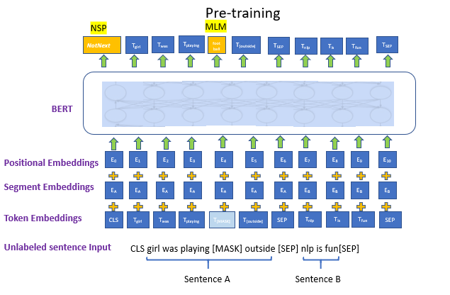
BERT 的 input是一条文本。文本中的每个词(token)我们都通过 embedding 矩阵 把它表示成了向量的形式。
embedding = token_embedding(将单个词转变为词向量) + position_embedding(位置编码,用于表示 token 在输入序列中的位置) + **segment_emebdding(**非必须,在 bert 中用于表示每个词属于哪个句子)。
在 VIT 中,同样存在 token_embedding 和 postion_emebedding。
在 Bert 中,我们同时做 2 个训练任务:
- Next Sentence Prediction Model(下一句预测):input 中会包含两个句子,这两个句子有 50% 的概率是真实相连的句子,50% 的概率是随机组装在一起的句子。我们在每个 input 前面增加特殊符
<cls>,这个位置所在的 token 将会在训练里不断学习整条文本蕴含的信息。最后它将作为 “下一句预测” 任务的输入向量,该任务是一个二分类模型,输出结果表示两个句子是否真实相连。 - Masked Language Model(遮蔽词猜测):在 input 中,我们会以一定概率随机遮盖掉一些 token(
<mask>),以此来强迫模型通过 Bert 中的 attention 结构更好抽取上下文信息,然后在 “遮蔽词猜测” 任务重,准确地将被覆盖的词猜测出来。
就和这次讲的 ViT 一样, BERT也只是重点放在特征的提取,同样也最多适用于分类任务。
ViT model design
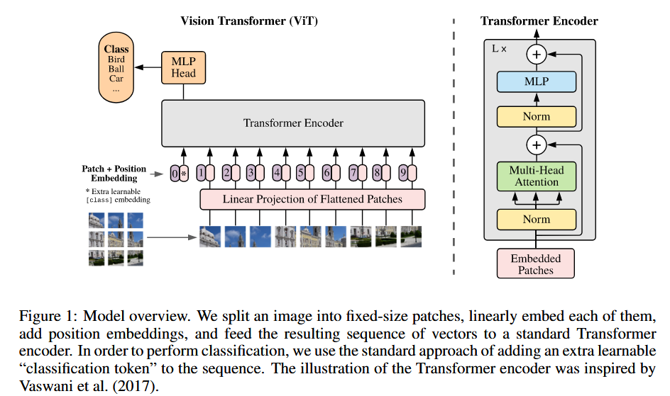
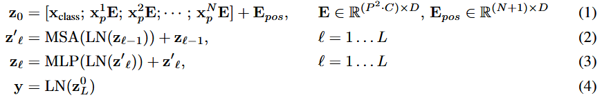
标准transformer接受 1D序列的 embedding (实际整体是2D)。为了针对 2D 序列的图片,要把图片扁平为 2D 的patch。将 HxWxC 的图片转换为 Nx(P^2xC) 的patch,注意是把 图片尺寸 HxW 切分成 P^2 的小块。
- patch embeddings: 之后为了转换为 embedding,将每个patch扁平化,并用linear层映射到embedding,类似于bert的 [cls] token,我们也需要用一个token,来作为最终的整体图片表示,这个 token 最终的标表征用于分类任务,实现起来就是定义一组可学习参数。transformers 里源码是定义 (1,1,hs) 的矩阵,FWD时会在batch维度扩展,再在第二维度(序列维度)上拼接。
1 | # init |
- position embedding: 另外将 position embedding添加到 patch embedding中以保留位置信息。我们使用标准可学习的1D位置嵌入,因为我们没有观察到使用更高级的2D感知能position embedding的性能提高,源码里除了正常图片的处理外,还有非正常大小图片的处理,大概就是将原本的 PE 插值化到目标图片的大小。
1 | # add positional encoding to each token |
- transformer blocks: 之后整体就和正常 transformer 一样了,都是 attention 和MLP的叠加,最后有一个分类head,是由MLP在预训练时间和微调时间的单个线性层的MLP实现的。
通常,我们在大型数据集上预先培训VIT,并对(较小)下游任务进行微调。为此,我们删除了预训练的预测头,并连接一个初始化为0的d×k的FFN,其中k是下游类的数量。比预训练更高的分辨率进行微分解通常是有益的。在喂食较高分辨率的图像时,我们保持patch大小相同,从而导致较大的有效序列长度。ViT可以处理任意序列长度(直至记忆约束),但是,预训练的position embedding可能不再有意义。因此,我们根据原始图像中的位置,对预训练的position embedding进行2D插值。
ViT CNN 混合模型
原文在最后还提出了混合结构,作为原始图像patch的替代方法,可以先从CNN的特征图中形成输入序列。在此混合模型中,patch embeddings 应用于从CNN特征图中提取的patch,相当于替代 linear 层提取特征。
As an alternative to raw image patches, the input sequence can be formed from feature maps of a CNN (LeCun et al., 1989). In this hybrid model, the patch embedding projection E (Eq. 1) is applied to patches extracted from a CNN feature map. As a special case, the patches can have spatial size 1x1, which means that the input sequence is obtained by simply flattening the spatial dimensions of the feature map and projecting to the Transformer dimension. The classification input embedding and position embeddings are added as described above.
虽说 ViT 是作为替代 CNN 的方法,但用 CNN 和这个不矛盾,由于这一步只是输入预处理阶段,和主体模型没有关系。
Transformers ViT 微调
预下载数据集和模型
1 | export HF_ENDPOINT="https://hf-mirror.com" |
loading dataset - beans
1 | from datasets import load_dataset |
1 | DatasetDict({ |
每个样本包含三个特征:
- image:一个 PIL 图像对象
- image_file_path:图像文件的路径,类型为字符串,该路径对应的图像已被加载为 image
- labels:一个 datasets.ClassLabel 特征,这里会以整数形式表示每个样本的标签
1 | ex = ds['train'][400] |
1 | {'image_file_path': '/home/albert/.cache/huggingface/datasets/downloads/extracted/967f0d9f61a7a8de58892c6fab6f02317c06faf3e19fba6a07b0885a9a7142c7/train/bean_rust/bean_rust_train.148.jpg', |
打印下图片
1 | image = ex['image'] |
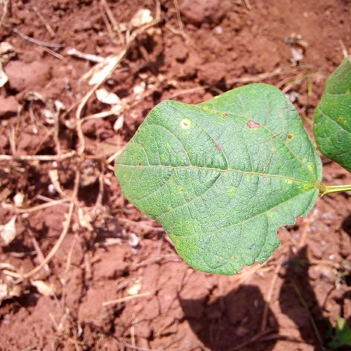
打印出该样本对应的类别标签。可以使用 ClassLabel 提供的 int2str 函数来实现,该函数可以将类别的整数表示转换为对应的字符串标签
1 | labels = ds['train'].features['labels'] |
1 | ClassLabel(names=['angular_leaf_spot', 'bean_rust', 'healthy'], id=None) |
loading ViT Image Processor
在训练 ViT 模型时,输入图像会经过特定的变换处理。如果对图像应用了错误的变换,模型将无法理解其所看到的内容!
为了确保应用正确的图像变换,我们将使用与预训练模型一同保存的配置来初始化一个 ViTImageProcessor。在本例中,使用的是 google/vit-base-patch16-224-in21k 模型
可以直接打印 ImageProcessor 来显示其 config
1 | from transformers import ViTImageProcessor |
1 | ViTImageProcessor { |
要处理一张图像,只需将其传递给图像处理器的 __call__ 函数即可。该函数会返回一个字典,其中包含 pixel_values,即图像的数值表示,可直接输入到模型中。
默认情况下返回的是 NumPy 数组,但如果添加参数 return_tensors='pt',则会返回 PyTorch 张量。
1 | ret = processor(image, return_tensors='pt') |
1 | {'pixel_values': tensor([[[[ 0.7882, 0.6706, 0.7098, ..., -0.1922, -0.1294, -0.1765], |
Processing the Dataset
接下来就要批量将 dataset 里的 image 转换为数值,我们直接利用 ViT 的 ImageProcessor。我们定义这个函数,仅返回训练所需的数据,即 1. 数值化的图片 2.分类标签
1 | def process_example(example): |
1 | {'pixel_values': tensor([[[[-0.5686, -0.5686, -0.5608, ..., -0.0275, 0.1843, -0.2471], |
map 返回的数据结构会将 PyTorch tensor 自动转换为 Python list(tolist()),以保证结果是 JSON 可序列化的。
1 | prepared_ds = ds.map( |
1 | ds['train'] |
1 | Dataset({ |
1 | prepared_ds['train'] |
1 | Dataset({ |
Training and Evaluation
数据已经处理完毕,现在你可以开始搭建训练流程了。本教程使用的是 Hugging Face 的 Trainer,但在此之前我们需要完成以下几项准备工作:
- 定义一个
collate函数:用于将一个 batch 的数据整理成模型可以接受的格式。 - 定义评估指标:在训练过程中,模型需要根据预测准确率进行评估,因此你需要定义一个
compute_metrics函数来计算这一指标。 - 加载预训练模型检查点:你需要加载一个预训练的检查点,并正确配置它以便进行训练。
- 定义训练配置:包括超参数设置、保存策略、日志输出等。
data collator 里再次将数据转换为 tensor,因为 dataset.map 默认还是会把 tensor 改为 list
1 | import torch |
1 | collate_fn([prepared_ds['train'][1], prepared_ds['train'][1]])['pixel_values'].shape |
1 | torch.Size([2, 3, 224, 224]) |
我们利用 evaluate 的 accuracy 函数来计算分类准确率
1 | import numpy as np |
现在让我们加载预训练模型。在初始化时,我们会传入 num_labels 参数,以便模型构建一个具有正确输出单元数量的分类头。同时,我们还会提供 id2label 和 label2id 的映射关系,以便在将模型推送到 Hugging Face Hub 时,能够在界面中显示可读的标签名称。
1 | from transformers import ViTForImageClassification |
1 | num of labels: 3 |
1 | from transformers import TrainingArguments |
1 | from transformers import Trainer |
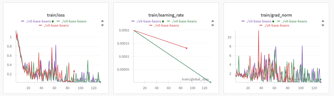
1 | train_results = trainer.train() |
1 | ***** train metrics ***** |
1 | metrics = trainer.evaluate(prepared_ds['validation']) |
1 | ***** eval metrics ***** |
infer
推理很简单了,直接把某个 image 通过 ImageProcessor 处理下图片为 tensor,接着 forward 到 model 即可,得到 logit 后再 argmax 就得到了预测类别。
1 | ex = ds['test'][0] |
1 | {'image_file_path': '/home/albert/.cache/huggingface/datasets/downloads/extracted/807042d188eb9a5d1d9a4179867e5b93eea6ed98d063904065fe40011681df29/test/angular_leaf_spot/angular_leaf_spot_test.0.jpg', |
1 | with torch.no_grad(): |
1 | torch.Size([1, 3]) |